Three Ethical Issues Related to Credit Score

By Sam Koslowsky, Senior Analytic Consultant, Harte Hanks

A reasonable credit score and its accompanying benefits provide an avenue for success today, far more than it has in the past. Of course, looking for a home, or a new car, or that premium credit card, requires the lender to conclude that you are credit-worthy.

But these scores, many believe,  are indicative of various personality traits. “Employers, insurers and even landlords regularly pull the applicants’ credit, already treating it as a proxy for a vague sort of approximation of your diligence, honesty and character. Consumer groups have raised questions about the use of credit as a way to assess things like people’s ethics, arguing that the two aren’t necessarily related.”1 You don’t need to ever borrow anything. It does not matter. Your credit score will follow you around.

While there are many noteworthy issues surrounding machine learning in credit scoring, I wanted to spend a few moments discussing three of them. And these topics were quite similar to the ones I had previously tackled when I began my career in credit scoring several decades ago.

Specifically, I wanted to briefly review the following:

• Negotiating a biased population-Reject inference
• A measurement criterion typically used in the credit scoring world, but less so in other machine learning applications-the KS statistic
• Some opportunities and challenges-the Data landscape

To construct a machine learning algorithm that distinguishes between ‘good’ (those that repay loans) and ‘bad’ customers, the researcher must use data that is available from previously accepted applicants. This, of course, makes sense. You model with what you have. And we have the known good or bad behaviors of these customers.

But wait a minute. How about the rejected applicants? The status of the rejected applicants cannot be identified, as they were never customers. Thus, no knowledge of their behavior is available.

As the resulting model is intended to be used on all applicants, not just the approved ones, we are left with a flawed view of future applicants, a bias, that can be a significant issue. How then do we deal with this dilemma?

Enter reject inference. Similar to other classification algorithms, to formulate a credit scoring model, we need to know the membership of the groups-the ‘good’ (those repaying their obligations), and the ‘bad’ (those who have not). However, as we alluded to above, there is no such information available for rejected applications. You see, we cannot be certain, to which category an applicant would have belonged, had he been accepted. The Reject Interference methods are designed to incorporate ‘inferences’ that identify what might have happened. Once this is accomplished, these ‘new’ records can be included in the model development sample.

These techniques, which have been used for decades, while providing a method to proceed with the analysis, nevertheless, often do not provide a total comfort level. Let’s briefly consider the dominant approaches.

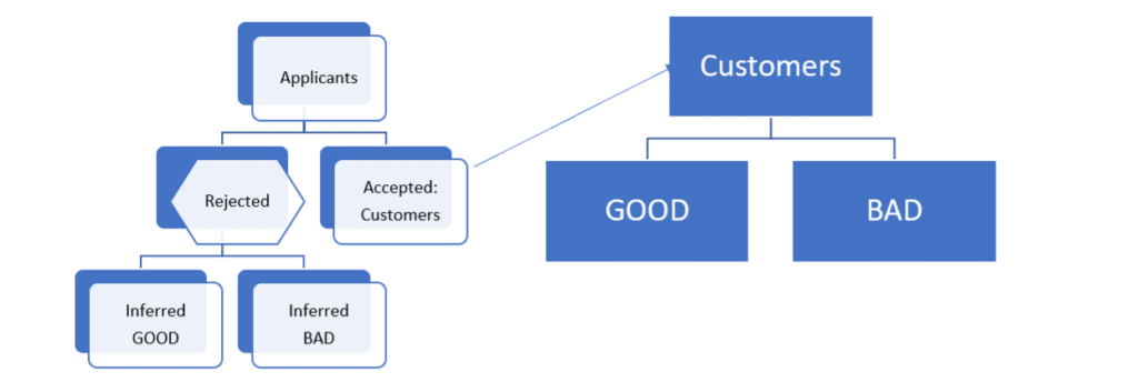
Look at the diagram below. This approach involves developing an algorithm on the accepted applicants-the customers. This appears on the right-hand side. This algorithm, although not designed to, is then used to predict the probabilities of repayment for the rejected applications (the hexagon box on the left-hand side). A cut-off value is established. Rejects are assessed as “good” or “bad” based on an agreed to cut-off score. Finally, an expanded file of approved and rejected applications is used to re-estimate the algorithm. This approach is referred to as the hard cut-off method.

An alternative approach referred to as fuzzy augmentation is somewhat similar. The resulting model computed from the accepted universe is used to predict the probability of going ‘bad’ and ‘good’ for the rejected applications, as depicted in the following diagram.

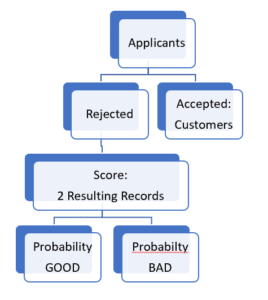
Each rejected applicant is replicated into two observations and given a weighted “good” and “bad” value, based on a probability of being “good” or “bad”, as depicted below.

2 Rejected applicants
convert to 4 records

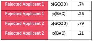
The weighted rejects are then added to the original accept population, and the combined data set is used to construct a new machine learning model.

The most straightforward tactic is to construct a machine learning credit scoring model by only utilizing the accepted applications! Essentially, this school of thought maintains that the rejected applications can be treated as ‘missing’. No one will argue with the simplicity of the method. And many maintain that analyzing the data this way provide more than adequate results! Not all researchers agree.

Other approaches do exist to address the rejected applications. They are, however, comparable to the above. But I do hope that you sense how we confront this issue.

Reject inference, after all these many years, is still a matter of dispute in the credit analytics community. Does it improve results? It depends on who you ask. Some argue, incorporating reject inference may be associated with overfitting, and result in the lack of ability, to generalize to a broader population. As you can expect, not all agree.

So how do these machine learning models perform?

In many classification problems, analysts typically use the ROC Curve and ROC AUC score as criteria of how well the resulting algorithms perform. Essentially, if lower scores are associated with actual lower probabilities, and higher score correlates with higher actual probabilities, we are in good shape.

In credit scoring, we have a similar metric. Credit data scientists enjoy using the Kolmogorov-Smirnov (KS) test.

Let’s proceed with an example to demonstrate how to compute the KS statistic. Below the following table, you will find a description of the calculations.

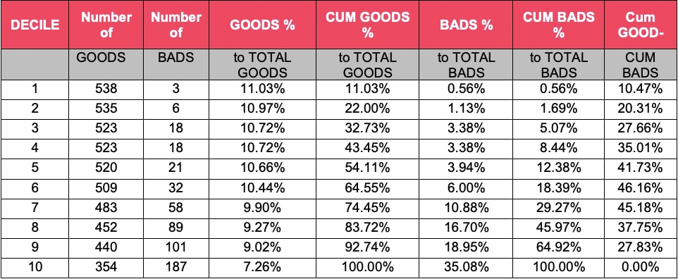
Score the development sample with the model, and rank the file from high score (probability of repaying loan) to low score

1. Divide the file into 10 equal groups-deciles (column titled ‘DECILE’)
2. Note the number of GOODS and BADS in each of the deciles. (columns labeled ‘Number of Goods and column labeled ‘Number of BADS’)
3. Record the number of GOODs in each decile as a percent of all GOODS (column labeled ‘GOODS as a % to Total GOODS’)
4. Create a cumulative column of GOODS to all GOODS (thru decile 1, thru decile 2, thru decile 3, etc.) (column labeled ‘ CUM GOODS as a % to Total GOODS’)
5. Record the number of BADS in each decile as a percent of all BADS (column labeled ‘BADS as a % to Total BADS’)
6. Create a cumulative column of BADS to all BADS (thru decile 1, thru decile 2, thru decile 3, etc.) ) (column labeled ‘ CUM BADS as a % to Total BADS’)
7. Subtract ‘7’ above from ‘5’ above. The maximum difference is the KS statistic, highlighted.

The higher the KS, the better discriminatory power. Although there does not appear to be universal agreement at to what the ‘ideal’ score should be, many opine that it should be in the first 3-4 deciles, and the value should range from 40 thru 70.

The benefit of using this statistic, I believe, is twofold.

• the ROC AUC score ranges from 0.5 to 1.0, while KS statistics extend from 0.0 to 1.0. Managers may find it difficult to understand intuitively that 0.5 is a poor score for ROC AUC, while 0.75 is “only” a medium one.
• The KS may be easier to calculate

So, we have briefly discussed the potential bias in model development, and several reject inference technologies to combat this issue. Then we moved to the KS metric that is often used in credit machine learning exercises. Finally, a thought on some challenges and opportunities.

The techniques employed for credit scoring have increased in complexity since I was first involved decades ago. No surprise here. More traditional statistical analyses have migrated to state-of-the-art approaches such as artificial intelligence, including machine learning algorithms such as random forests, gradient boosting, support vector machines and neural networks. The opportunities of using advanced methods for these efforts may include increased precision in the underlying models, productivity improvement from mechanization of procedures, and equally important, a real possibility of a better customer experience.

All these improvements require quality and predictive data. The result of falling below the cutoff score would translate into being rejected for credit. Whether it’s a loan from the bank, or a mortgage from your lender, or a credit card, the denial of credit can have a major impact on an individual’s way of life. Typically, a lender has used the data that usually appears on an application-age, gender, income, family status, etc. In some cases, the acceptance of more modern techniques has also expanded the variety of data that may be deemed applicable for machine learning credit models.

But hold on. Are we talking about Facebook, Twitter, TikTok, or LinkedIn, for example? These platforms collect information about members’ friends, preferences and other behaviors. Are there issues with employing this data? By tapping into these unconventional data sources, perhaps a better evaluation of the applicant can be made.

We are not done. How about all the smart devices? Should they be incorporated? Can anyone see any ethical or legal implications? We have not even mentioned privacy. It appears to me, that while machine learning applied to these data, may provide better models, serious questions may still remain.

 

1 https://time.com/3595130/credit-score-health/